As a robot navigates in an unknown environment, it must take measurements and simultaneously estimate its own location and the shape of the world around it. This is called the SLAM (simultaneous localization and mapping) problem Here, I consider the monocular SLAM case, where the robot is armed with just a single RGB camera. I simplify the problem further by only building a small map within the view of a single camera image. My task, then, is to take in a few camera images of a scene and reconstruct its 3D geometry.

It turns out that you can represent this 3D reconstruction task as an optimization problem and set it up in a few lines of Python. My approach is based on the depth map estimation step of the LSD-SLAM algorithm, but it is significantly simpler. The cost of this simplicity is that my approach is slower to run.

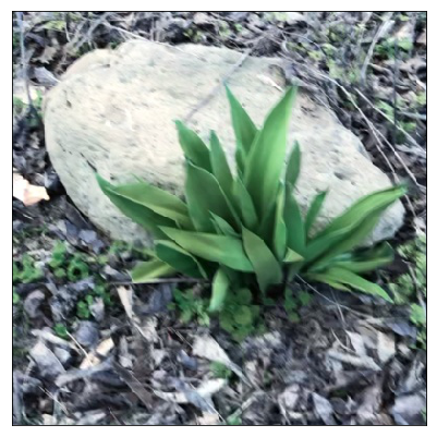
Given a scene of a rock and a plant, my algorithm recovers the 3D geometry of the scene and the positions of the cameras that photographed it from five different positions. The algorithm jointly optimizes over the estimated camera poses and scene geometry to produce the scene below.

This animation shows the depth map being refined over the course of optimization. Brighter pixels are estimated to be closer to the camera.

Background

This post assumes that you are familiar with basic linear algebra and gradient descent. You don’t need to know about any simultaneous localization and mapping (SLAM) algorithms to understand this post. My algorithm uses a Lie Algebra representation of SE(3) to represent camera poses. In this post, I treat that machinery as a black box, though if you want to understand it, I recommend Ethan Eade’s document on Lie algebras for representing transformations.

Why we care about depth

A depth image contains at each pixel the distance from the camera to that point in the scene. This small 3D model of the world in the camera’s view is useful for building larger maps and localizing a robot within them. The quickest way to get a depth image is to use an RGB-Depth camera like a Kinect or RealSense. However, such hardware is more expensive than standard RGB cameras and not nearly as ubiquitous. In low-cost robotics applications, for instance, we are interested in ways of getting the same 3D information about the world with clever algorithms and cheap RGB cameras.

Depth from RGB images

In the absence of hardware for instantly producing RGB-D images, you can produce depth images by imaging the same scene from several perspectives and then reconstructing its 3D geometry. This method does not require knowledge of the exact positions that the different frames were taken from. This sets it apart from methods that assume you have a calibrated stereo pair of cameras. As we will see, the algorithm works with unknown camera poses on unknown scenes.

If we assume the scene is rigid, we can reason about what the scene’s 3D structure must be given that the camera saw a certain set of images. For instance, in the images in the figure below, the green cylinder moves more in the image between frames than the blue cube does because it is closer to the camera.

The algorithm

This algorithm takes as input a set of images like those in the scene above and arbitrarily designates one to be the “reference image.” The algorithm outputs the distance from the reference camera plane to each point in the scene, along with the camera poses from which each photo was taken.

The heart of this algorithm is the warp operation that takes an image taken by one camera and renders it as though it were taken from another position. It is aware of the scenes geometry and so captures effects like parallax. If we correctly estimate scene geometry and all camera poses, we should be able to warp the images taken from one view to another view and end up with an image that looks the same.

In my algorithm, I warp all the scene images into the view of the reference camera. I then optimize the estimated camera poses and scene geometry until all the scene images look as similar as possible to the reference image.

The diagram below gives a high level overview of this approach.

The image warp is a differentiable operation that takes as input

• The depth image from the reference camera’s view
• Some image of the scene \(I\)
• A transform that takes the reference camera’s pose and moves it to the pose of the camera that took the scene image \(I\)

and outputs a warped image where the pixels in \(I\) have been moved to their locations in the view of the reference camera. In a nutshell, we know how the camera projects world points into the image plane, we know how far each reference image pixel is from the reference camera, and we have estimated the transform between the reference camera and the camera that took \(I\). Given all that, we can calculate a correspondence between pixels in \(I\) and pixels in the reference image. By resampling \(I\) according to this correspondence, we get an image of the pixels in \(I\) from the reference camera’s point of view.

The figure above illustrates warping one pixel between camera views by inferring its location in 3D space. This correspondence is found for all pixels in order to warp one view into another. The warp operation is differentiable, allowing us to easily optimize the depth and pose variables it takes as input using gradient descent.

The formula for the warp given

• \(p\), a pixel location in the reference image
• \(d(p)\), a function mapping a pixel location \(p\) in the reference image to the depth value at that location
• \(\textbf{T}\), a homogeneous transformation matrix representing the transform from some camera’s frame to that of the reference image

is

gives us the location of pixel \(p\) in the view of the reference camera. The homogeneous transform \(T\) is computed from the representation of the camera poses using the method in Ethan Eade’s document, which I implement for Tensorflow in tf_lie.py.

Once \(I\) is warped into the reference camera view, we need some way of measuring how well this warped image approximates the reference image. This will tell us how closely our depth map and camera poses match the true values. I use a photometric loss to measure the difference between two images. There are many possible functions we could use here. I simply compute a Huber loss on the raw RGB values. The Huber loss has a couple of nice properties. First, it is dead simple. Second, the Huber loss is a robust loss, so if some pixels are way off due to occlusion or specular highlights in one image, our total loss will not be hugely affected. If \(ref(p)\) is the reference image’s color at position \(p\) and \(I(p)\) is an image \(I\)’s color at position \(p\), then our cost function is

For clarity, the function above elides summing over the r, g, and b channels of each pixel.

As a note, the iteratively reweighted least squares optimization scheme proposed in the LSD-SLAM paper can be seen as finding the minimum of the robust distance metric between images, although they don’t frame it this way. Details on that can be found in Ethan Eade’s document on Gauss-Newton optimization.

Given the ability to represent camera poses and warp images, solving for the depth map and camera poses is a simple optimization problem to set up. Given a few images \(I\) and a reference image, we take a sum over the photometric loss for each \(I\) given the depth estimate and camera pose estimate for that image. We can now jointly optimize the poses and depth using gradient descent to minimize the sum of photometric losses.

The video below shows the whole optimization process in action. The points on the lower right are the estimated locations of the cameras. Each pixel in the scene is represented as a point that moves closer to or farther away from the reference camera (the blue point) according to its depth value over the course of optimization. Notice how the camera images are arranged in a smooth arc. That is because I took these images from a video, during which I made a smooth sweeping motion with the camera.

An implementation in tensorflow

My implementation can be found here.

That repo contains

• An ipython notebook that generates a depth map using my approach
• A directory of images of the rock and plant scene
• tf_lie.py, a utility for handling SE(3) transformations in Tensorflow which operates on tensors for which the last dimension represents SE(3) elements
• image_warping.py which implements the image warp described above

The heart of the implementation is this snippet, which is in the notebook. Here it is pared down for clarity, omitting some casting and other cruft.

depth =  tf.abs(tf.Variable(tf.ones([400,400]))) +.1

cost = 0.0

for scene_image in scene_images:
    # pose representation for the cameras that took each scene image
    translation_representation = tf.Variable([[0.01, 0.01, 0.01]])
    rotation_representation = tf.Variable([[0.01, 0.01, 0.01]])

    warped_scene_image = warp_image(scene_image, depth,
                                    translation_representation,
                                    rotation_representation)

    cost += tf.losses.huber_loss(reference_image, warped_scene_image)
    
optimizer = tf.train.AdamOptimizer(learning_rate=.005).minimize(cost)

init = tf.global_variables_initializer()
sess = tf.Session()
sess.run(init)
for _ in range(2000):
    sess.run(optimizer)

In about a dozen lines of python, you can capture the essence of the depth map estimation algorithm.

1. First, initialize the depth map to be all ones and constrain depth to be positive.
2. Define the cost to be the robust Huber metric between the reference image and the scene image warped into the reference view.
3. Minimize the loss by adjusting the camera poses and the depth map using gradient descent.

The rest of the code in the notebook is data setup and visualization.

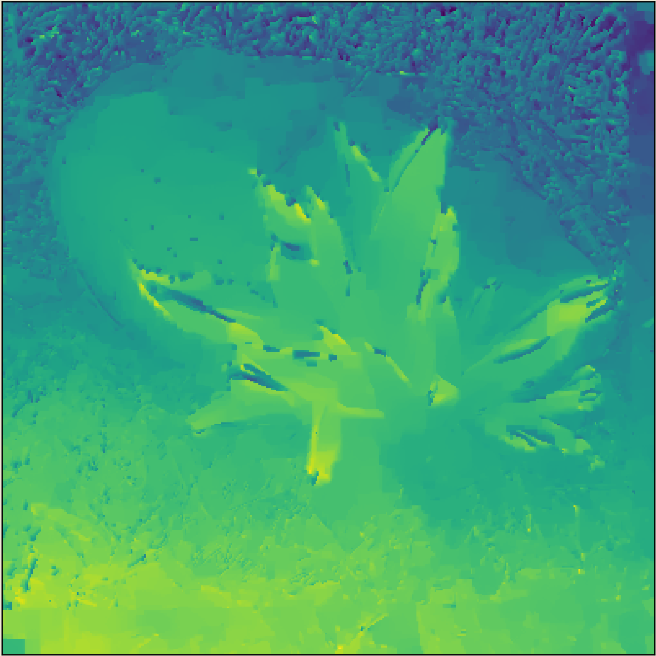
In this project, I have allowed myself one hack: I include a total variation term in the cost function. Total variation measures the amount of discontinuity in the depth map and so encourages the depth map to be smooth. This term makes the results look better and something like it is often used in depth estimation, but is not very principled. For instance, it penalizes flat surfaces that are tilted with respect to the camera, and a surface like grass that truly has lots of depth discontinuity will be penalized. A slightly better approach would be to penalize the curvature of the depth map, but that is a slippery slope of heuristics and hand-tuning.

This approach yields the depth map below. It looks reasonable, but has obvious blocky artifacts caused by the total variation term encouraging flat regions to form.

Refining the depth map using a “deep image prior”

In the approach above, I represent each pixel as an independent depth value, and introduce some regularity through a total variation term. While this is important for reducing high-frequency noise in the depth map, it creates artifacts of its own. This motivated me to explore other forms of regularization.

In the deep image prior paper, the authors consider a related problem of denoising natural images. The authors train a u-net style architecture to take a corrupted image and simply reproduce it as the network’s output. This task is trivial since the network need only memorize a single data sample. However, the authors show that the network tends to memorize “natural” image structure more easily than noise and other artifacts. The u-net serves as a useful prior in the sense that it more readily memorizes the structure the authors are interested in preserving from the image.

I experimented with representing the depth map as the output of a u-net rather than as independent values at each pixel. The u-net architecture takes as input the reference image and downsamples it before resampling it up to its original resolution. At each resolution, there is a residual path allowing some high-resolution spatial information to be preserved. I found that this approach works surprisingly well and is insensitive to the exact hyperparameters of the u-net such as number of downsampling operations or the number of filters.

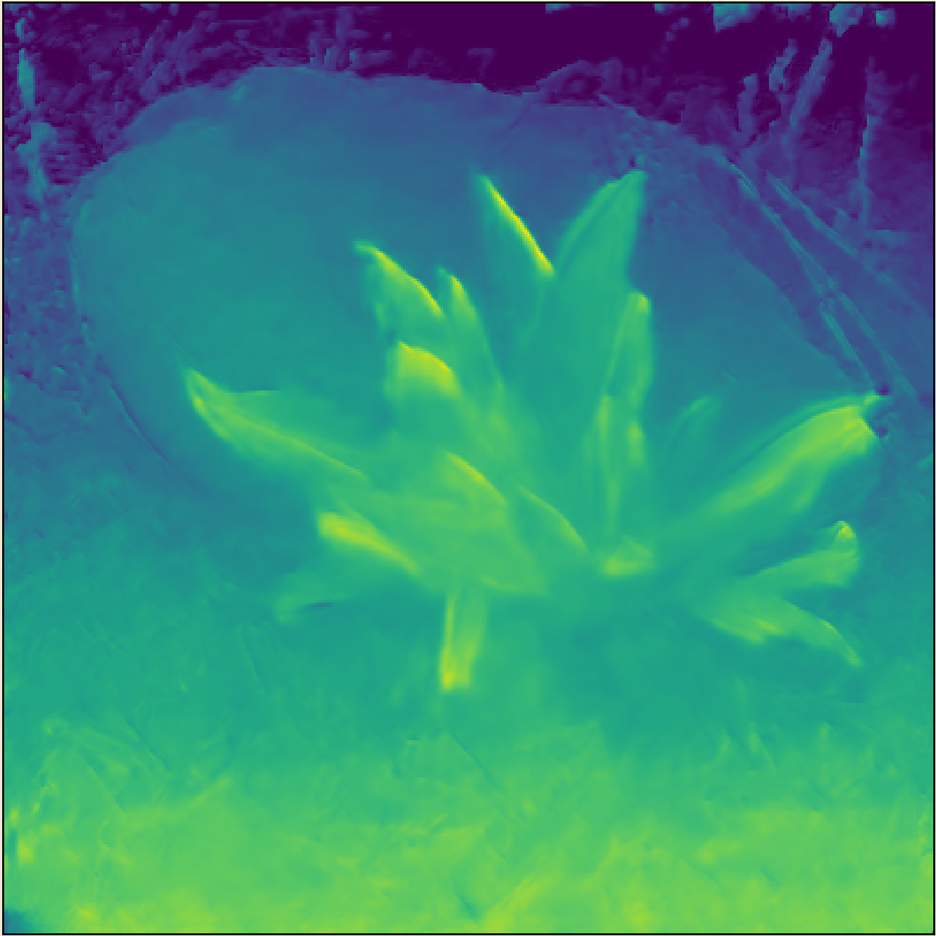
An example of a depth map produced with this approach is shown below. This depth map is overall much smoother, but also recovers fine details such as the twigs to the upper right of the rock. Following the intuition of the deep image prior paper, I imagine that the network tends to default to producing smooth regions because they are easiest to represent. However, the architecture is highly expressive, and so can output arbitrarily fine detail when forced to do so by the cost function. This is closer to regularizing the depth map toward some abstract ideal of “parsimony” rather than toward a particular type of simplicity, such as geometric smoothness.

The diagram below shows that this approach differs from the previous one only in terms of the representation of the depth map.

Conclusion

For this scene of a plant and a rock on some leaf litter,

my approach which represents the depth map using a u-net produces this depth map:

While that depth map is not perfect, it was produced with a very simple optimization setup. Once you have utilities for manipulating camera poses (tf_lie.py) and doing image warping (image_warping.py), the depth problem can be solved in about a dozen lines of tensorflow code. This stands in stark contrast to much of the work in the literature, where real-time requirements shift the focus from the fundamental simplicity of the optimization problem at hand to the complex approaches one needs to use in order to gain speed.