Conditional Variational Autoencoders

Introduction

When I started working on understanding generative models, I didn’t find any resources that gave a good, high level, intuitive overview of variational autoencoders. Some great resources exist for understanding them in detail and seeing the math behind them. In particular “Tutorial on Variational Autoencoders” by Carl Doersch covers the same topics as this post, but as the author notes, there is some abuse of notation in that article, and the treatment is more abstract then what I’ll go for here. Here, I’ll carry the example of a variational autoencoder for the MNIST digits dataset throughout, using concrete examples for each concept. Hopefully by reading this article you can get a general idea of how Variational Autoencoders work before tackling them in detail.

Goal of a Variational Autoencoder

A variational autoencoder (VAE) is a generative model, meaning that we would like it to be able to generate plausible looking fake samples that look like samples from our training data. In the case of the MNIST data, these fake samples would be synthetic images of handwritten digits. Our VAE will provide us with a space, which we will call the latent space, from which we can sample points. Any of these points can be decoded into a reasonable image of a handwritten digit.

Structure of a VAE

The goal of any autoencoder is to reconstruct its own input. Usually, the autoencoder first compresses the input into a smaller form, then transforms it back into an approximation of the input. The function used to compress the data is usually called an “encoder” and the function used to decompress the data is called a “decoder.” Those functions can be neural networks, which is the case we’ll consider here.

A standard autoencoder

Standard autoencoders can work well if your goal is simply to reconstruct your input, but it won’t work as a generative model, because picking a random input V’ to the decoder won’t necessarily cause the decoder to produce a reasonable image. V’ could be far away from any input the decoder has seen before, and so the decoder may never have been trained to produce reasonable digit images when given an input like V’.

We need some way of ensuring that the decoder is prepared to decode any input we give it into a reasonable digit image. To do this, we’ll need to predefine the distribution of inputs that the decoder should expect to see. We’ll use a standard normal distribution to define the distribution of inputs the decoder will receive.

A standard normal distribution. This is how we would like points corresponding to MNIST digit images to be distributed in the latent space.

We would like to train the decoder to take any point sampled from this distribution and return a reasonable digit image.

The decoder of a variational autoencoder

Now we need an encoder. In a traditional autoencoder, the encoder takes a sample from the data and returns a single point in the latent space, which is then passed into the decoder. In a variational autoencoder, the encoder instead produces a probability distribution in the latent space.

The encoder of a variational autoencoder

The latent distributions it outputs are gaussians of the same dimensionality as the latent space. The encoder produces the parameters of these gaussians.

So we have an encoder that takes in images and produces probability distributions in the latent space, and a decoder that takes points in the latent space and returns artificial images. So for a given image, the encoder produces a distribution, a point in the latent space is sampled from that distribution, and then that point is fed into the decoder which produces an artificial image.

A variational autoencoder

The Structure of the Latent Space

I said earlier that the decoder should expect to see points sampled from a standard normal distribution. But now I’ve stated that the decoder receives samples from non-standard normal distributions produced by the encoder. These two things aren’t at odds, though, if points sampled from the encoder still approximately fit a standard normal distribution. We want a situation like this:

where the average of different distributions produced in response to different training examples approximate a standard normal. Now the assumption that the decoder sees points drawn from a standard normal distribution holds.

Obviously we need some way to measure whether the sum of distributions produced by the encoder “approximates” the standard normal distribution. We can measure the quality of this approximation using Kullback-Leibler divergence. Kullback-Leibler divergence essentially measures how different two probability distributions are. This is treated in more depth in Doersch’s tutorial.

Training a VAE with The Reparametrization Trick

In the VAE described above, there is a random variable in the network between the input and output. There’s no way to backpropagate through a random variable, which presents the obvious problem that you’re now unable to train the encoder. To solve this problem, the VAE is expressed in a different way such that the parameters of the latent distribution are factored out of the parameters of the random variable, so that backpropagation can proceed through the parameters of the latent distribution. Concretely, N(μ,Σ) = μ + Σ N(0, I) when the covariance matrix Σ is diagonal, which it is in our case. But this is treated in more depth in other articles. The important takeaway is that a VAE can be trained end-to-end using backprop. But since there is still an element of randomness involved, instead of being called stochastic gradient descent, the training process is called stochastic gradient variational Bayes (SGVB).

Conditional Variational Autoencoder

So far, we’ve created an autoencoder that can reproduce its input, and a decoder that can produce reasonable handwritten digit images. The decoder cannot, however, produce an image of a particular number on demand. Enter the conditional variational autoencoder (CVAE). The conditional variational autoencoder has an extra input to both the encoder and the decoder.

A conditional variational autoencoder

At training time, the number whose image is being fed in is provided to the encoder and decoder. In this case, it would be represented as a one-hot vector.

To generate an image of a particular number, just feed that number into the decoder along with a random point in the latent space sampled from a standard normal distribution. Even if the same point is fed in to produce two different numbers, the process will work correctly, since the system no longer relies on the latent space to encode what number you are dealing with. Instead, the latent space encodes other information, like stroke width or the angle at which the number is written.

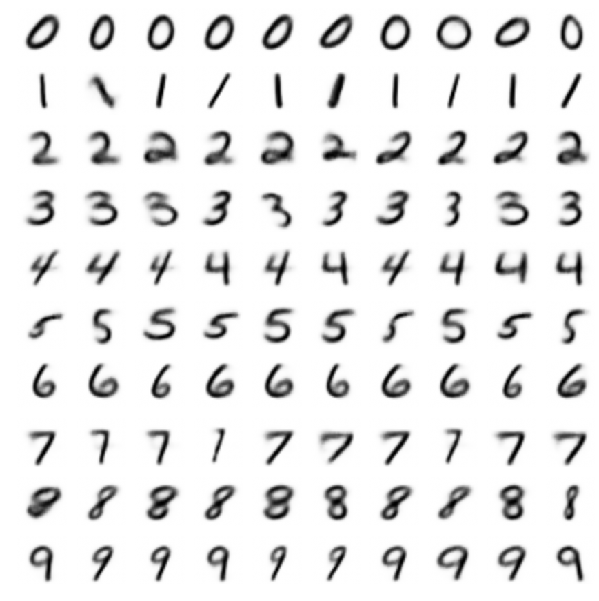
A variational autoencoder generating images according to given labels

The grid of images below was produced by fixing the desired number input to the decoder and taking a few random samples from the latent space to produce a handful of different versions of that number. As you can see, the numbers vary in style, but all the images in a single row are clearly of the same number.