In the two years after publishing this, I worked on refining this algorithm to power a real-time world generator, called Generate Worlds, and it lets you design your own 2D and 3D tile sets and explore the worlds they generate in first-person. I have a post that describes it, and it’s available for purchase on itch.io.

Here’s Generate Worlds in action:

Introduction

This post describes two algorithms for creating complex procedural worlds from simple sets of colored tiles and constraints on the placements of those tiles. I will show that by carefully designing these tile sets, you can create interesting procedurally generated content, such as landscapes with cities, or dungeons with complex internal structure. The video below shows the system creating a procedural world based on the rules encoded in 43 colored tiles.

The image below shows the tile set that generated the world in the video above. The world is annotated to assist in the exercise of imagination required to see it as an actual environment.

We will define a tiling as a finite grid where one of those tiles lies in each grid square. We will further define a valid world as one where the colors along the edges of adjacent tiles must be the same.

This is the only concrete rule for a tiling: tile edge colors must match up. All the higher level structure flows from this.

A valid tiling looks like this:

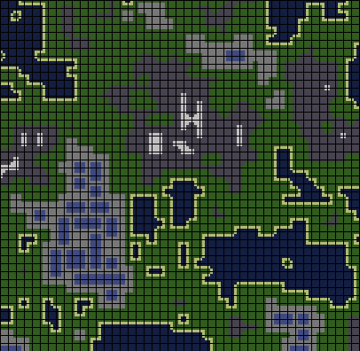
This is a tiling which is supposed to represent a map with water, beaches, grass, towns with buildings (blue rectangles), and snow capped mountains. The black lines show borders between tiles.

I think this is an interesting way to describe and create worlds because very often, procedural generation algorithms take a top-down approach. L-systems, for instance, rely on a recursive description of an object where the top level, large details are determined before lower level ones. There is nothing wrong with this approach, but I think that it is interesting to create tile sets that are only able to encode simple low level relationships (e.g., ocean water and grass must be separated by a beach, buildings can only have convex, 90 degree corners) and see high level patterns emerge (e.g. square buildings).

Tiling is an NP complete Constraint Satisfaction Problem

For the reader familiar with constraint satisfaction problems (CSPs), it will already be clear that tiling a finite world is a CSP. In a CSP, we have a set of variables, a set of values that each variable can take on (called its domain), and a set of constraints. For us, the variables are locations in the map, the domain of each variable is the tile set, and the constraints are that tiles must match along their edges with their neighbors.

Intuitively, the problem of correctly creating a nontrivial tiling is hard because the tile sets can encode arbitrary, long range dependencies. Formally, this is an NP complete constraint satisfaction problem when we consider tile sets in general. A naive algorithm for creating tilings would exhaustively search the space of tilings and run in exponential time. The hope is that we can create interesting worlds using tile sets that are solvable using search accelerated by heuristics. The other option is to create tilings that are nearly correct, but may have a small number of incorrect placements. I have found two algorithms that work well with some interesting tile sets, and I describe them below.

Method 1: Greedy Placement with Backjumping

Keep choosing random locations and place valid tiles there. If you get stuck, remove some and try again.

Initialize the entire map to UNDECIDED

while UNDECIDED tiles remain on the map
    if any valid tile can be placed on the map
      t <- collection of all possible valid tile placements
      l <- random selection from t weighted by tile probabilities
      place l on the map
    else
      select a random UNDECIDED tile and set all its neighbors to UNDECIDED

The first approach I took to creating a tiling from a tile set is to simply start with the entire grid in an undefined state, and to iteratively place a random tile in a location where it is valid, or, if no locations are valid, set a small region on near an undefined tile to be undefined and continue greedy placement. The “greedy placement” is the strategy of placing a tile as long as all its edges line up with existing tiles, without regard for whether this placement will create a partial tiling that cannot be completed without removing existing tiles. When such a situation arises, and we cannot place any more tiles, we must remove some previously placed tiles. But we can’t say which are ideal to remove, because if we could solve that problem, we could probably also have solved the problem of placing tiles in a smart way in the first place. To give the algorithm another chance at finding a valid tiling for a given area, we set all the tiles around the location that undefined and continue with the greedy placement strategy. Eventually, the hope is, a valid tiling will be found, but this is not guaranteed. The algorithm will continue to run until a valid tiling is found, which may be forever. It has no ability to detect when a tile set is unsolvable.

There is no guarantee that this algorithm will halt. A simple tile set with two tiles that share no colors would cause this algorithm to loop forever. An even simpler case would be one tile with different colors on the top and bottom. It might make sense to somehow check for tile sets that cannot produce valid tilings. We might say that a tile set is certainly valid if it can tile an infinite plane. In some cases it is clearly possible to prove or disprove whether a tile set can tile an infinite plane, but the problem turns out to be undecidable in general. Therefore, it is up to the designer of the tile set to create one which can yield a valid tiling.

This algorithm is unable to find good solutions for the dungeon tile set in the video at the top of this post. It performs well on simpler tile sets. We would like to solve more complex tile sets where many types of transitions between tiles are possible and lots of rules (e.g. roads begin and end at buildings) are encoded. We need an algorithm that is able to look ahead and take make tile placements while being somehow aware of what options that placement will leave open for future placements. This will allow us to efficiently solve complex tile sets.

From a constraint satisfaction perspective

This algorithm is a backjumping random search. At each step, we attempt to assign a single variable. If we cannot, we unassign a variable and all the variables which are connected by constraints to it. This is called backjumping, which differs from backtracking, where we unassign only one variable at a time. In backtracking, we generally unassign variables in the reverse of the order we assigned them, but with backjumping we unassign variables according to the structure of the problem at hand. It makes sense that if we can’t place any tile at a particular location, we should change the placement of neighboring tiles, since their placement created an unsolvable situation. Backtracking may instead cause us to unassign variables that are spatially far away but happened to be assigned recently.

This search does not employ any local consistency method. That is, we make no attempt to place tiles that won’t cause an unsolvable situation later on, even as soon as one step of search in the future. It may be possible to accelerate search by keeping track of the effects that a placement will have on possible placements a few tiles away. Hopefully, this will keep our search from spending so much time undoing its work. This is what the next algorithm does.

Method 2: Most Constrained Placement with Local Information Propagation

Maintain a probability distribution over tiles at each location, making nonlocal updates to these distributions when a placement decision is made. Never backtrack.

Next, I’ll describe an algorithm which is guaranteed to halt and produces better looking results for all the tile sets I have tried. It is also able to produce nearly-valid tilings for much more complicated tile sets. The tradeoff is that this algorithm does not guarantee that its output is always a valid tiling. The Optimizations section describes optimizations that help this technique run fast even over large tile sets and maps.

The difficulty of creating a valid tiling is largely determined by the number of transitions necessary to get between two tile types. A simple tile set might contain only sand, water, and grass. If grass and water cannot touch, then a transition to sand will be necessary between the two. This is a simple case that the previous algorithm can solve easily. A more complex case might involve many nested levels of tile types. For instance, you might have deep water, water, sand, grass, high plain, mountain, and snow cap. Seven transitions would need to be present in the map for all of these types to appear, assuming that these types cannot touch except in the order I stated them. Further complexity can be introduced by creating tiles that naturally create long-distance dependencies between tiles, like roads that must start and end at certain types of tiles.

Intuitively, it makes sense that an algorithm for this problem should have some ability to “look ahead” and consider at least a few transitions out what the consequences of its placement choices might be. In order to do this, the tile map is considered to be a probability distribution over tiles at each location. When the algorithm places a tile, it updates the probability distributions around that tile in response to the placement so that the probabilities of nearby tiles that are likely to be compatible with the placement are increased.

For example, if a water tile is placed on the map, the tiles next to it must contain some water. The tiles next to those tiles might also contain water, but there are other possibilities, such as grass if a beach was placed next to the original water. The farther we get from the placed tile, the more types of tiles become possible. To make concrete use of this observation, we can count the number of ways that we can arrive at each tile placement near the original tile. In some cases, only a single sequence of transitions can cause one tile to transition to another over a given distance. In other cases, there could be many possible transition sequences. Once we have placed a tile, we can determine the probability distributions of tiles at nearby locations by counting the number of ways we can transition from the tile we have placed to nearby tiles. The “look ahead” that the algorithm performs is tracking these transition counts and treating them as probability distributions from which to select future tiles to place.

At each time step, the algorithm examines all non-decided tile locations, each of which is a probability distribution over tiles, and selects one location to place a tile. It selects the distribution from the map with the lowest entropy. Low entropy multinomial distributions tend to have their probability concentrated in a few modes, so placing these first means placing tiles we already have some constraints for. This is why the algorithm fills in tiles near tiles that are already decided first.

This is the most effective algorithm I have managed to implement for this problem, and it has the added advantage of lending itself to nice visualizations as it runs. It may be possible to improve this algorithm by adding some form of backtracking. If an invalid location exists in the final tiling, undoing nearby tile placements and then resampling from the resulting distributions at their locations may allow a fix to be found for the final tiling. Of course, if you were determined to always keep searching until a valid tiling is found, you would lose the bounded run time guarantee we have now.

Optimizations

The core operation of this method is updating the probabilities around a placed tile. One approach would be to count the possible transitions outward from a placed tile each time a tile is placed. This would be very slow, since many transition pairs would need to be considered for each map location to which the new probabilities are propagated. One obvious optimization is not to propagate across the entire map. A more interesting optimization is to cache the effect that each tile placement will have on the locations around it, so that each tile placement merely does a lookup to see what type of changes to the neighboring probabilities a placement makes, and then apply that change via some simple operation. I will describe my technique for doing this below.

Imagine a tile were placed on an otherwise empty map. This placement would update the probabilities of tiles nearby. We can think of these updated distributions as having a prior distribution which is informed by previous placements. If multiple tiles are placed, this prior is a joint distribution. I approximate the posterior given this joint prior as the product of the distributions given each placement in the past.

To implement this, I imagine that when a tile is placed on an empty map, it induces a significant change in the distributions in the map nearby. I call these updates the sphere of the tile, as in, the sphere of influence the tile projects around it when it is placed on an empty map. When two tiles are placed near each other, their spheres interact to create the final distributions that are affected by both placements. Considering that many tiles may be placed near a given undecided location, there could be a large number of interacting constraints that would make a counting based approach to finding the probability of different tiles appearing at that location slow. What if we instead only consider a simple model of the interaction between the precomputed spheres of the tiles that have already been placed?

When a tile is placed, I update the probability map by elementwise multiplying the distribution of that tile’s sphere at each location in the map with the distribution already stored in that location in the map. It may be helpful to consider an example of what this might do to the distribution map. Say a given location in the map currently has a distribution that considers grass and water likely, and we place a water tile next to that location. The water tile’s sphere will have a high probability of water right next to the water tile, and a low probability of grass. When we multiply these distributions together elementwise, the probability of water in the result is high, because it is the product of two large probabilities, but the probability of grass will become low, because it is the product of the high probability stored in the map with the low probability stored in the sphere.

This strategy allows us to efficiently approximate the effect that each tile placement should have on the probability map.

Relationship to Wave Function Collapse

This strategy was inspired by the animations from the Wave Function Collapse project. The pictures above look similar to those from Wave Function Collapse, but there are a few key differences between the strategies. This method uses the same basic principle of placing a piece of the world and then eliminating other placements that are now ruled out. In Wave Function Collapse, this is done by discretely removing placement possibilities across the whole image each time a pixel is updated. In my method, the updates are all local, and rather than discretely removing possible placements, I reweight the probability distributions at the nearby locations. Since my updates are local, most of the world is totally blank early in generation. In Wave Function Collapse, you’ll notice updates immediately start far away from the “collapsed” region of the generated texture. The advantage of only doing local updates is that the algorithm is fast even for large worlds.

An advantage of using continuous distributions rather than discrete ones to represent the possible placements is fault tolerance. If Wave Function Collapse eliminates all possible placements at a location, it quits and restarts from scratch. Since my method maintains a fuzzy notion of valid placements, it can still select a tile that fits most of its neighbors even when no strictly valid placement is possible.

From a constraint satisfaction perspective

To solve constraint satisfaction problems efficiently, it often makes sense to keep track of what assignments of other variables become impossible when a particular variable is assigned. This is known as “enforcing local consistency.” Enforcing some kind of local consistency helps prevent you from assigning a value to a variable then assigning an incompatible value to a nearby value right away and being forced to backtrack. Such transformations are under the umbrella of constraint propagation methods in the CSP literature. In this algorithm, we are propagating information through a small area of the map each time we place a tile about what tiles can or cannot appear nearby. If we place a mountain tile, for instance, we know that there can’t be an open ocean tile only two tiles away, so the probability of ocean at all locations on the map two tiles from the placement is set to zero. This local information is recorded in the spheres discussed above.

By reducing the number of possible assignments of nearby tiles, we significantly reduce the search space the algorithm needs to handle after with each placement. We know that in that small neighborhood, all probabilities of tiles appearing that are incompatible with the places tile are zero. This is equivalent to removing those values from the domains of the variables at those locations. This means that each pair of neighboring locations in the region around the placement has some tile in its domain that is compatible with some tile still in its neighbors domain. When two variables are connected by a constraint in a CSP problem and their domains contain only values that could satisfy the constraint, they are said to be arc consistent, so this method is really an efficient arc consistency enforcing strategy.

In a CSP, the “most constrained” variable in a given partial assignment is the one with the fewest possible values remaining in its domain. The idea of placing a tile at the location of the lowest entropy distribution in the map is analogous to assigning a value to the most constrained variable in a CSP, which is a common variable ordering heuristic when solving CSPs by search.

Manipulating Tilings by Changing Tile Selection Probabilities.

So far, I’ve talked about only about how to create valid tilings, but beyond being valid, there might be other properties we might like a tiling to have. For instance, we might like it to have a certain ratio of one tile type to another, or we might like to ensure that it is not all one uniform type of tile, even if such a tiling is valid. To accomplish this, both the algorithms I describe take as input a base probability associated with each tile. The higher this probability, the more likely that tile should be in the final tiling. Both algorithms make random choices over collections of tiles, and I simply weight these random choices by the base tile probabilities.

Below, you can see how this is used. By adjusting the probability of the solid water tile appearing, I can adjust the size and frequency of water features on the map.

Make Your Own Tile Sets

In short,

• clone my repo on github
• Download Processing 2.2.1
• use Processing to open wangTiles.pde and click the play button

Using the code I’ve put on github, you can create your own tilesets using an image editor, and see how the tiling solver creates worlds with them. Simply clone the repo and edit the image named tiles.png, then use Processing to run wangTiles.pde to see an animation of the map being generated.

The Tile Set Specification

The tiles are laid out on a grid of 4x4 cells. Each cell contains a colored tile in the upper left 3x3 region, and the remaining 7 pixel contain metadata about the tile. The pixel below the center of the tile can be set to pure red to comment that tile out of the set. The solvers will never include it in a map. The upper pixel to the right of the tile can be set to pure black to add all 4 rotations of the tile to the tile set as well. This is a nice shorthand when you want to add something like a corner, which can reasonably exist in 4 orientations. Finally, the most important piece of markup is the pixel below and to the left of the tile. This controls the base probability of that tile appearing in the map. The darker the pixel is, the more likely that tile is to appear.

Related Work

Many people have explored Wang tiles, which are tile sets with colored edges that must match in edge color with tiles they are placed next to, just like the tiles I have talked about here.

The Wave Function Collapse project by @ExUtumno explores creating textures from examples, including textures that represent maps of simple dungeons. That algorithm maintains a map boolean vectors representing possible pixel assignments and progressively removes possible assignments from consideration when they are discovered to be incompatible with pixels placed so far. As is pointed in the paper WaveFunctionCollapse is constraint solving in the wild, this information propagation step is the same as the well-known AC-3 algorithm for local consistency originally introduced in 1977. The system as a whole is effectively a greedy constraint satisfaction solver with some modifications to its tie breaking to help the result texture match the statistics of the input texture. This is a different approach than those discussed here, which don’t use canonical local consistency methods like AC-3, and in the case of the second algorithm, maintain a continuous, as opposed to discrete, distribution over possible placement decisions at each location.

Wave Function Collapse is predated by Paul Merrell’s Model Synthesis algorithm, which appears to also be an AC-3-based constraint satisfaction system, although AC-3 is not mentioned in this paper or Merrell’s thesis. Merrell considers the problem of generating 3D models from 3D tiles with adjacency constraints, like those I have in 2D above. Merrel’s work includes an interesting sampling strategy where he starts with a trivial solution and progressively replaces sections of it using his constraint satisfaction algorithm, maintaining a consistent model at each step.

Conclusion and Acknowledgments

Enforcing local rules to create high level structure, such as having a rule that roads have no dead ends enforcing the fact that roads must lead from some non-road location to another, is an interesting perspective on the problem of procedural generation. A surprising range of interesting rules can be encoded this way. The quality of the resulting tilings is highly dependent on the solver, however, so a fruitful direction for future work would be improving the algorithms that do the tiling. I have not explored using genetic algorithms, simulated annealing, or general purpose constraint satisfaction algorithms for this task yet. Any of these might yield a tile set solver that is able to handle a wide range of tile sets with minimal parameter tuning.

I would like to thank Cannon Lewis and Ronnie McLaren for helpful discussions during this project. Ronnie came up with many interesting ideas about how to encode interesting behavior in the tiles. The meothd 2 algorithm resulted from a conversation with Cannon on Wave Function Collapse, and his advice was instrumental in creating the efficient approximate algorithm that I described in here.